
Authors:
(1) Goran Muric, InferLink Corporation, Los Angeles, (California [email protected]);
(2) Ben Delay, InferLink Corporation, Los Angeles, California ([email protected]);
(3) Steven Minton, InferLink Corporation, Los Angeles, California ([email protected]).
Table of Links
2 Related Work and 2.1 Prompting techniques
3.3 Verbalizing the answers and 3.4 Training a classifier
4 Data and 4.1 Clinical trials
4.2 Catalonia Independence Corpus and 4.3 Climate Detection Corpus
4.4 Medical health advice data and 4.5 The European Court of Human Rights (ECtHR) Data
7.1 Implications for Model Interpretability
7.2 Limitations and Future Work
A Questions used in ICE-T method
5 Experiments
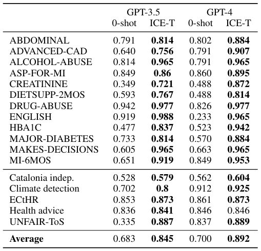
We performed the experiments on a set of binary classification tasks on datasets from various domains, as described in the previous section.
To generate the secondary questions, we employed a large language model. Prompting it only once, we obtained a set of n secondary questions, which we accepted as provided, without any selection or modification. More specifically, we used the following prompt for creating all secondary questions:
Return {n} yes/no questions that would be useful to ask if you were trying to determine the answer to the following question: "{primary_question}"
where n is the number of additional questions we want to generate and primary_question is the primary question used to obtain the main information from the document. Note that in all our experiments n = 4. That means that for each document we use one primary and four secondary questions that are treated equally when prompting the LLM. Thus, for each document we collect five answers from the LLM that are then verbalized (assigned a numerical value) in the next step. To generate the secondary questions for all our experiments we use OpenAI’s gpt-4-0125-preview model. To collect the answers in our experiments we use two generations of OpenAI’s models: gpt-4-0125-preview (Achiam et al., 2023) and gpt-3.5-turbo-0125 (Brown et al., 2020).
To choose the best classifier, we train several different classification algorithms. These include K-Nearest Neighbors, Decision Trees, Random Forest, Gaussian Naive Bayes, Multinomial Naive Bayes, AdaBoost, and XGBoost. We use a 5-fold cross-validation on our training data and also perform a grid search to fine-tune the parameters for each classifier. After training, we test them on a hold-out test set and choose the classifier that gives us the highest Micro F1 score (µF1). Note that one can also adjust the training process to optimize for a specific performance metric if needed for a particular application. To perform these experiments, we used the scikit-learn library in Python.
Micro F1 score is particularly useful in datasets where some classes are significantly underrepresented, and where traditional metrics might give a misleading picture of model performance. It treats every instance as equally important, thereby giving a more accurate measure of the model’s performance across the board. To calculate the µF1, we use the following formula:
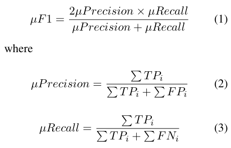
and T P, F P and F P represent number of true positives, false positives and false negatives respectively
Additionally, we conducted a sensitivity analysis to enhance our understanding of the relationship between the number of features and the improvement of the µF1. This analysis helps determine the requisite number of secondary questions to attain a desired µF1. For each dataset, we started by creating n = 9 secondary questions and using the gpt-3.5-turbo-0125 model to generate responses for each sample. The outputs from the large language model were then transformed into 10-dimensional feature vectors. Subsequently, we constructed a series of simple Random Forest classifiers, starting with a single feature and incrementally adding more features up to ten. Given the random selection of features for classification, we repeated the experiment 100 times. We computed the µF1 for each iteration and dataset. The findings are detailed in Section 6 and illustrated in Figure 3.
This paper is